[playground] Julia Turing.jl : Bayesian Cognitive Modeling - Some examples of data analysis
bayesian cognitive modeling chapter 5 with julia programming language
Github: https://github.com/quangtiencs/bayesian-cognitive-modeling-with-turing.jl
Bayesian Cognitive Modeling is one of the classical books for Bayesian Inference. The old version used WinBUGS/JAG software as the main implementation. You can find other implementations, such as Stan and PyMC, in the below link. I reimplemented these source codes with Julia Programming Language & Turing library in this tutorial.
- WinBUGS/JAGS (official) & Stan: https://bayesmodels.com/
- PyMC: https://github.com/pymc-devs/pymc-resources/tree/main/BCM
5.1 Pearson correlation
\mu_{1},\mu_{2} \sim \text{Gaussian}(0, 1/ \sqrt{.001}) \sigma_{1},\sigma_{2} \sim \text{InvSqrtGamma} (.001, .001) r \sim \text{Uniform} (-1, 1)
x_{i} \sim \text{MvGaussian} \left( (\mu_{1},\mu_{2}), \begin{bmatrix} \sigma_{1}^2 & r\sigma_{1}\sigma_{2} \\\ r\sigma_{1}\sigma_{2} & \sigma_{2}^2\end{bmatrix} \right)
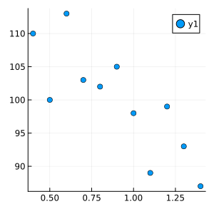
x = [[0.8, 102.0],
     [1.0, 98.0],
     [0.5, 100.0],
     [0.9, 105.0],
     [0.7, 103.0],
     [0.4, 110.0],
     [1.2, 99.0],
     [1.4, 87.0],
     [0.6, 113.0],
     [1.1, 89.0],
     [1.3, 93.0]]

m = transpose(reduce(hcat, x));
freq_correlation = cor(m[:, 1], m[:, 2])

@model function PearsonCorrelationModel1(x)
    r ~ Uniform(-1., 1.)
    mu ~ filldist(Normal(0.0, 1. / sqrt(0.001)), 2)
    lambda ~ filldist(truncated(Gamma(0.001, 1 / 0.001), lower=1e-7, upper=1000), 2)
    sigma = 1 ./ sqrt.(lambda)
    cov = [1/lambda[1]         r*sigma[1]*sigma[2];
           r*sigma[1]*sigma[2] 1/lambda[2]]
    for i in eachindex(x)
        x[i] ~ MultivariateNormal(mu, cov)
    end
enditerations=10_000
burnin=500
chain = sample(PearsonCorrelationModel1(x), NUTS(1000, 0.9; init_ϵ=0.02), iterations, burnin=burnin
, init_theta=(r=-0.7, mu=[0.9, 100], lambda=[9, 0.02]))
bayes_corr_plot = histogram(chain[:r], label=false, alpha=0.1, normalize=true)
height = max(filter(e -> !(isnan(e)), bayes_corr_plot[1][1][:y])...)
density!(chain[:r], label="Posterior Correlation", size=(600, 200))
println("Freq Correlation:", freq_correlation)
println("Posterior R Estimation:", mean(chain[:r] |> collect))
plot!([freq_correlation, freq_correlation], [0, height], label="Freq Correlation", linewidth=4, fmt=format)Sampling: 100%|█████████████████████████████████████████| Time: 0:00:01
Freq Correlation:-0.8109670756358504
Posterior R Estimation:-0.6949106643379455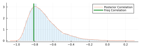

Chains MCMC chain (10000×1×1 Array{Float64, 3}):

Iterations        = 1001:1:11000
Number of chains  = 1
Samples per chain = 10000
Wall duration     = 7.67 seconds
Compute duration  = 7.67 seconds
parameters        = r
internals         =

Summary Statistics
  parameters      mean       std   naive_se      mcse         ess      rhat    ⋯
      Symbol   Float64   Float64    Float64   Float64     Float64   Float64    ⋯

           r   -0.6949    0.1667     0.0017    0.0021   5186.3199    0.9999    ⋯
                                                                1 column omitted

Quantiles
  parameters      2.5%     25.0%     50.0%     75.0%     97.5%
      Symbol   Float64   Float64   Float64   Float64   Float64

           r   -0.9148   -0.8141   -0.7305   -0.6141   -0.2717
5.2 Pearson correlation with uncertainty
\mu_{1},\mu_{2} \sim \text{Gaussian}(0, .001) \sigma_{1},\sigma_{2} \sim \text{InvSqrtGamma} (.001, .001) r \sim \text{Uniform} (-1, 1)
y_{i} \sim \text{MvGaussian} \left((\mu_{1},\mu_{2}), \begin{bmatrix}\sigma_{1}^2 & r\sigma_{1}\sigma_{2} \\\\ r\sigma_{1}\sigma_{2} & \sigma_{2}^2\end{bmatrix} \right) x_{ij} \sim \text{Gaussian}(y_{ij},\lambda_{j}^e)
x = [[0.8, 102.0],
     [1.0, 98.0],
     [0.5, 100.0],
     [0.9, 105.0],
     [0.7, 103.0],
     [0.4, 110.0],
     [1.2, 99.0],
     [1.4, 87.0],
     [0.6, 113.0],
     [1.1, 89.0],
     [1.3, 93.0]]
sigma_error = [0.03, 1.0]
# sigma_error = [0.03, 10.0]

m = transpose(reduce(hcat, x));
freq_correlation = cor(m[:, 1], m[:, 2])

@model function PearsonCorrelationModel2(x)
    r ~ Uniform(-1., 1.)
    mu ~ filldist(Normal(0.0, 1. / sqrt(0.001)), 2)
    lambda ~ filldist(truncated(Gamma(0.001, 1 / 0.001), lower=1e-7, upper=1000), 2)
    sigma = 1 ./ sqrt.(lambda)
    cov = [1/lambda[1]         r*sigma[1]*sigma[2];
           r*sigma[1]*sigma[2] 1/lambda[2]]

    y = Vector{Vector}(undef, length(x))
    for i in eachindex(x)
        y[i] ~ MultivariateNormal(mu, cov)
        x[i] ~ MvNormal(y[i], sigma_error)
    end
end

iterations=10_000
burnin=5_000

logger = Logging.SimpleLogger(Logging.Error)
chain = Logging.with_logger(logger) do
   sample(PearsonCorrelationModel2(x), NUTS(1000, 0.9; init_ϵ=0.02), iterations, burnin=burnin)
end

bayes_corr_plot = histogram(chain[:r], label=false, alpha=0.1, normalize=true)
height = max(filter(e -> !(isnan(e)), bayes_corr_plot[1][1][:y])...)
density!(chain[:r], label="Posterior Correlation", size=(600, 200))
println("Freq Correlation:", freq_correlation)
println("Posterior R Estimation:", mean(chain[:r] |> collect))
plot!([freq_correlation, freq_correlation], [0, height], label="Freq Correlation", linewidth=4, fmt=format)
Sampling: 100%|█████████████████████████████████████████| Time: 0:00:10
Freq Correlation:-0.8109670756358504
Posterior R Estimation:-0.707698754727043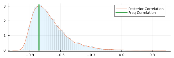
Chains MCMC chain (10000×39×1 Array{Float64, 3}):

Iterations        = 1001:1:11000
Number of chains  = 1
Samples per chain = 10000
Wall duration     = 14.61 seconds
Compute duration  = 14.61 seconds
parameters        = r, mu[1], mu[2], lambda[1], lambda[2], y[1][1], y[1][2],
y[2][1], y[2][2], y[3][1], y[3][2], y[4][1], y[4][2], y[5][1], y[5][2], y[6][1],
y[6][2], y[7][1], y[7][2], y[8][1], y[8][2], y[9][1], y[9][2], y[10][1], y[10][2],
y[11][1], y[11][2]
internals         = lp, n_steps, is_accept, acceptance_rate, log_density,
hamiltonian_energy, hamiltonian_energy_error, max_hamiltonian_energy_error,
tree_depth, numerical_error, step_size, nom_step_size

Summary Statistics
  parameters       mean       std   naive_se      mcse          ess      rhat  ⋯
      Symbol    Float64   Float64    Float64   Float64      Float64   Float64  ⋯

           r    -0.7077    0.1645     0.0016    0.0018    8325.4187    0.9999  ⋯
       mu[1]     0.9196    0.1103     0.0011    0.0011    8824.5770    0.9999  ⋯
       mu[2]    99.2518    2.6873     0.0269    0.0272    8605.3889    0.9999  ⋯
   lambda[1]     9.6645    4.2193     0.0422    0.0395   11030.1791    0.9999  ⋯
   lambda[2]     0.0164    0.0072     0.0001    0.0001   10264.5579    1.0006  ⋯
     y[1][1]     0.8008    0.0299     0.0003    0.0003   17468.1463    0.9999  ⋯
     y[1][2]   101.9749    0.9814     0.0098    0.0065   22015.0363    0.9999  ⋯
     y[2][1]     0.9993    0.0296     0.0003    0.0002   20131.5447    0.9999  ⋯
     y[2][2]    97.9950    1.0033     0.0100    0.0067   23034.7125    0.9999  ⋯
     y[3][1]     0.5078    0.0295     0.0003    0.0002   23658.7533    0.9999  ⋯
     y[3][2]   100.2488    0.9990     0.0100    0.0075   21035.4230    0.9999  ⋯
     y[4][1]     0.8967    0.0303     0.0003    0.0003   13896.6164    1.0001  ⋯
     y[4][2]   104.7986    0.9955     0.0100    0.0069   19690.0894    1.0000  ⋯
     y[5][1]     0.7022    0.0296     0.0003    0.0002   20837.7832    1.0001  ⋯
     y[5][2]   103.0138    0.9898     0.0099    0.0071   22622.8507    1.0000  ⋯
     y[6][1]     0.4042    0.0292     0.0003    0.0002   19468.6436    0.9999  ⋯
     y[6][2]   109.9443    0.9752     0.0098    0.0065   18272.1134    0.9999  ⋯
     y[7][1]     1.1946    0.0304     0.0003    0.0002   21935.2455    1.0000  ⋯
     y[7][2]    98.8367    0.9901     0.0099    0.0078   18614.5866    0.9999  ⋯
     y[8][1]     1.3978    0.0300     0.0003    0.0002   18379.3279    0.9999  ⋯
     y[8][2]    87.1597    0.9927     0.0099    0.0067   20195.1954    0.9999  ⋯
     y[9][1]     0.5984    0.0297     0.0003    0.0002   17940.5118    1.0001  ⋯
     y[9][2]   112.6867    0.9925     0.0099    0.0081   17646.8957    1.0000  ⋯
      ⋮           ⋮          ⋮         ⋮          ⋮          ⋮           ⋮     ⋱
                                                     1 column and 4 rows omitted

Quantiles
  parameters       2.5%      25.0%      50.0%      75.0%      97.5%
      Symbol    Float64    Float64    Float64    Float64    Float64

           r    -0.9236    -0.8272    -0.7429    -0.6258    -0.2935
       mu[1]     0.7075     0.8488     0.9173     0.9883     1.1435
       mu[2]    93.6298    97.6217    99.3438   100.9859   104.3339
   lambda[1]     3.2546     6.5745     9.0539    12.1124    19.6782
   lambda[2]     0.0057     0.0111     0.0153     0.0205     0.0331
     y[1][1]     0.7428     0.7805     0.8007     0.8208     0.8603
     y[1][2]   100.0329   101.3261   101.9774   102.6141   103.9200
     y[2][1]     0.9410     0.9793     0.9992     1.0192     1.0562
     y[2][2]    96.0241    97.3035    97.9938    98.6829    99.9415
     y[3][1]     0.4497     0.4876     0.5076     0.5278     0.5658
     y[3][2]    98.2955    99.5667   100.2461   100.9326   102.1994
     y[4][1]     0.8372     0.8763     0.8967     0.9170     0.9570
     y[4][2]   102.8479   104.1349   104.7939   105.4598   106.7453
     y[5][1]     0.6433     0.6823     0.7023     0.7220     0.7609
     y[5][2]   101.0435   102.3509   103.0184   103.6796   104.9578
     y[6][1]     0.3471     0.3846     0.4042     0.4241     0.4613
     y[6][2]   108.0433   109.2915   109.9499   110.5899   111.8738
     y[7][1]     1.1344     1.1742     1.1943     1.2150     1.2541
     y[7][2]    96.9020    98.1683    98.8344    99.5087   100.7409
     y[8][1]     1.3398     1.3775     1.3979     1.4182     1.4563
     y[8][2]    85.2048    86.5008    87.1558    87.8195    89.0989
     y[9][1]     0.5395     0.5787     0.5985     0.6181     0.6566
     y[9][2]   110.7736   112.0166   112.6787   113.3587   114.6394
      ⋮           ⋮          ⋮          ⋮          ⋮          ⋮
                                                       4 rows omitted
5.3 The kappa coefficient of agreement
\kappa = (\xi-\psi)/(1-\psi) \xi = \alpha\beta + (1-\alpha) \gamma \psi = (\pi_{a}+\pi_{b})(\pi_{a}+\pi_{c})+(\pi_{b}+\pi_{d})(\pi_{c}+\pi_{d}) \alpha,\beta,\gamma \sim \text{Beta} (1, 1)
\pi_{a} = \alpha\beta \pi_{b} = \alpha(1-\beta)
\pi_{c} = (1-\alpha)(1-\gamma)
\pi_{d} = (1-\alpha)\gamma
x \sim \text{Multinomial} ([\pi_{a},\pi_{b},\pi_{c},\pi_{d}],n)
# Influenza
x = [14, 4, 5, 210]

# Hearing Loss
# x = [20, 7, 103, 417]
# Rare Disease
# x = [0, 0, 13, 157]

@model function KappaCoefficientAgreement(x)
    alpha ~ Beta(1, 1)
    beta ~ Beta(1, 1)
    gamma ~ Beta(1, 1)

    pi1 = alpha * beta
    pi2 = alpha * (1 - beta)
    pi3 = (1 - alpha) * (1 - gamma)
    pi4 = (1 - alpha) * gamma

    xi = alpha * beta + (1 - alpha) * gamma

    x ~ Multinomial(sum(x), [pi1, pi2, pi3, pi4])

    psi = (pi1 + pi2) * (pi1 + pi3) + (pi2 + pi4) * (pi3 + pi4)
    kappa = (xi - psi) / (1 - psi)

    return (psi=psi, kappa=kappa)
end

iterations=10_000
burnin=5_000

model_kappa = KappaCoefficientAgreement(x)
chain = sample(model_kappa, NUTS(), iterations, burnin=burnin)
chains_params = Turing.MCMCChains.get_sections(chain, :parameters)
quantities = generated_quantities(model_kappa, chains_params);
Sampling: 100%|█████████████████████████████████████████| Time: 0:00:00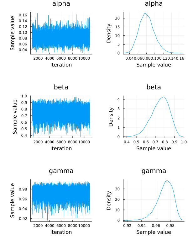
0.7357943807483934kappa = map(x -> x[:kappa], quantities)
h = histogram(kappa, size=(500, 300), alpha=0.2, normalize=true, label=false)
height = max(filter(e -> !(isnan(e)), h[1][1][:y])...)
density!(kappa, label="Posterior Kappa")
println("Freq:", kappa_cohen)
println("Mean Posterior:", mean(kappa))
plot!([kappa_cohen, kappa_cohen], [0, height], label="Freq Kappa", linewidth=4, fmt=format)Freq:0.7357943807483934
Mean Posterior:0.6981673531822107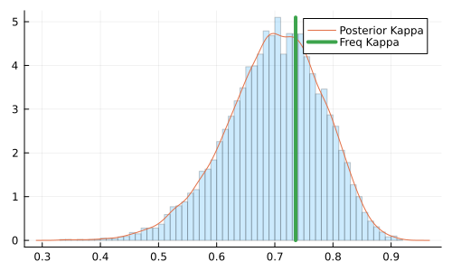
5.4 Change detection in time series data
\mu_{1},\mu_{2} \sim \text{Gaussian}(0, 1 / \sqrt{.001}) \lambda \sim \text{Gamma} (.001, .001) \tau \sim \text{Uniform} (0, t_{max})
c_{i} \sim \begin{cases} \text{Gaussian}(\mu_{1}, \lambda), & \text{if $t_{i} \lt \tau$} \\ \text{Gaussian}(\mu_{2}, \lambda), & \text{if $t_{i} \ge \tau$} \end{cases}
x = df.data
n = length(x)

@model function ChangePointTimeSeries(x, x_index)
    mu ~ MvNormal([0, 0], sqrt(1000) * ones(2))
    lambd ~ truncated(Gamma(0.001, 1 / 0.001), lower=1e-7, upper=1000)

    tau ~ Uniform(1, length(x))
    is_less_than_tau = x_index .< tau

    for i in eachindex(x)
        if is_less_than_tau[i] > 0
            x[i] ~ Normal(mu[1], 1/lambd)
        else
            x[i] ~ Normal(mu[2], 1/lambd)
        end
    end
end

iterations=2_000
burnin=1000

model_changepoint = ChangePointTimeSeries(x, eachindex(x) |> collect)
chain = sample(model_changepoint, NUTS(), iterations)
Sampling: 100%|█████████████████████████████████████████| Time: 0:00:50
Chains MCMC chain (2000×16×1 Array{Float64, 3}):
Iterations = 1001:1:3000
Number of chains = 1
Samples per chain = 2000
Wall duration = 53.36 seconds
Compute duration = 53.36 seconds
parameters = mu[1], mu[2], lambd, tau
internals = lp, n_steps, is_accept, acceptance_rate, log_density,
hamiltonian_energy, hamiltonian_energy_error, max_hamiltonian_energy_error,
tree_depth, numerical_error, step_size, nom_step_size
Summary Statistics
parameters mean std naive_se mcse ess rhat ⋯
Symbol Float64 Float64 Float64 Float64 Float64 Float64 ⋯
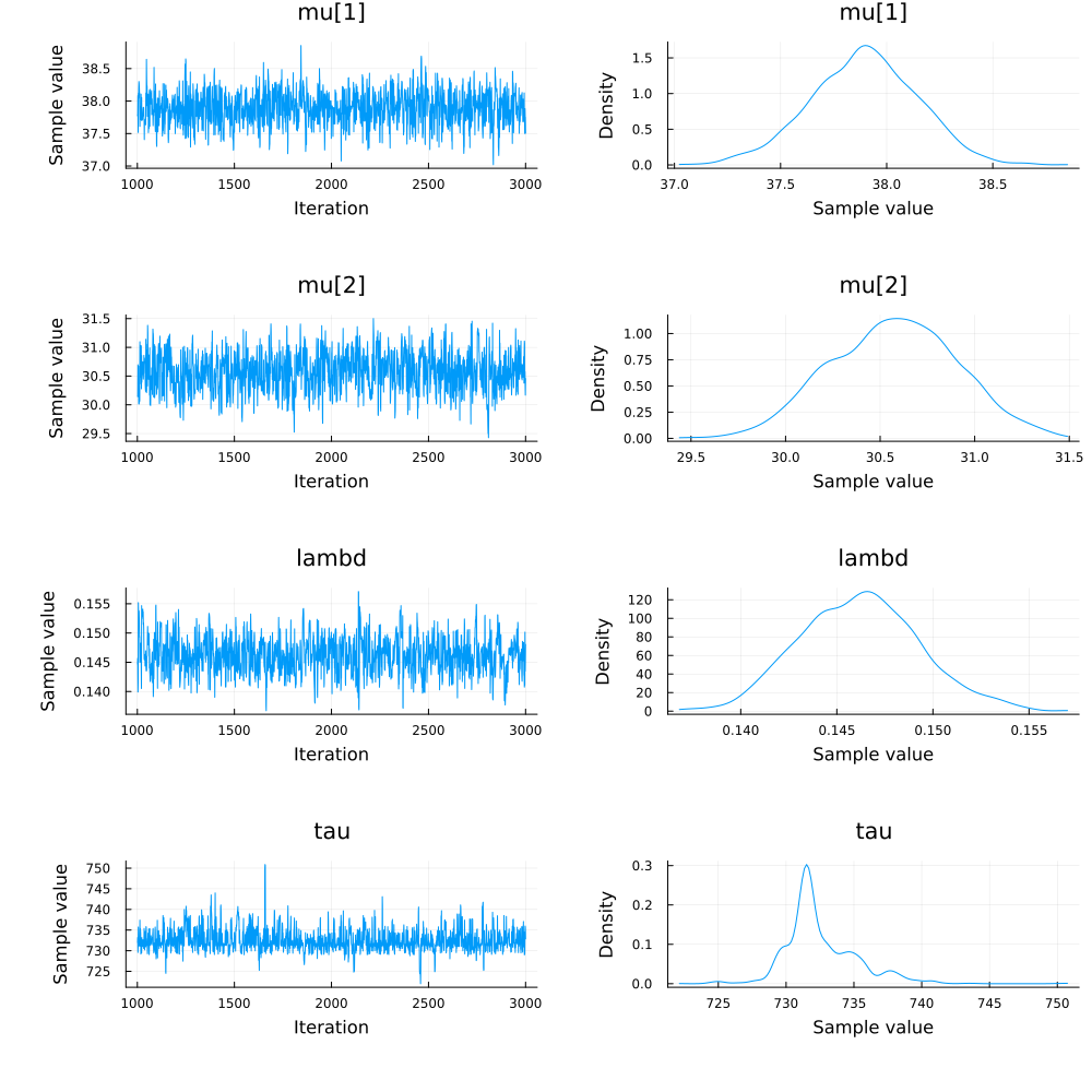
mu[1] 37.8935 0.2519 0.0056 0.0081 848.0341 0.9998 ⋯
mu[2] 30.5731 0.3347 0.0075 0.0141 511.1892 1.0075 ⋯
lambd 0.1462 0.0031 0.0001 0.0002 515.3547 0.9999 ⋯
tau 732.5357 2.6711 0.0597 0.1192 527.5883 1.0063 ⋯
1 column omitted
Quantiles
parameters 2.5% 25.0% 50.0% 75.0% 97.5%
Symbol Float64 Float64 Float64 Float64 Float64
mu[1] 37.3788 37.7242 37.8973 38.0655 38.3694
mu[2] 29.9319 30.3368 30.5773 30.8057 31.2169
lambd 0.1405 0.1440 0.1462 0.1483 0.1527
tau 729.0119 731.1409 731.7966 733.9456 738.6237p1 = plot(eachindex(x) |> collect, x, size=(800, 300), label=false, alpha=0.5)
mu1 = mean(chain[:"mu[1]"])
mu2 = mean(chain[:"mu[2]"])
mean_tau = mean(chain[:tau])
plot!([1, mean_tau], [mu1, mu1], label=L"\overline{\mu_1}", linewidth=4, color="red")
plot!([mean_tau, length(x)], [mu2, mu2], label=L"\overline{\mu_2}", linewidth=4, color="red")
plot!([mean_tau, mean_tau], [mu1, mu2], label=L"\overline{\tau}", linewidth=4, color="green")
p2 = histogram(chain[:tau], size=(800, 300), label=L"\tau", color="green")
plot(p1, p2; layout=(2,1), size=(800, 500), fmt=format)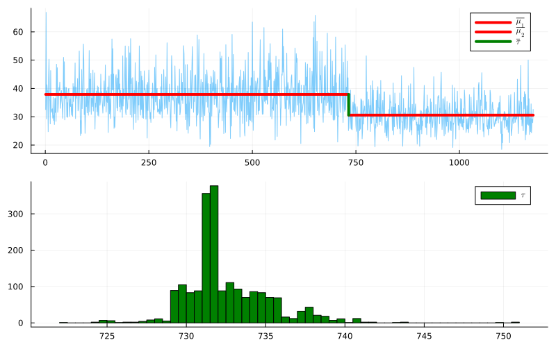
5.5 Censored data
\theta \sim \text{Uniform}(0.25, 1) z_{i} \sim \text{Binomial}(\theta, n) 15 \le z_{i} \le 25, \text{if} \; y_{i} = 1
x = 30
n = 50
nfails = 949
range_unobs = 15:25 |> collect
z = 30

function censor_likelihood(n, p, range_unobs, nfails)
    return loglikelihood(Binomial(n, p), range_unobs) * nfails
end

@model function ChaSaSoon(x, n, range_unobs, nfails)
    theta ~ Uniform(0.25, 1.0)
    x ~ Binomial(n, theta)
    Turing.@addlogprob! censor_likelihood(n, theta, range_unobs, nfails)
end

iterations=10_000
burnin=1000

model_chachasoon = ChaSaSoon(x, n, range_unobs, nfails)
chain = sample(model_chachasoon, NUTS(), iterations, burnin=burnin)
plot(chain, size=(800,300), left_margin=10Plots.mm, bottom_margin=10Plots.mm, fmt=format)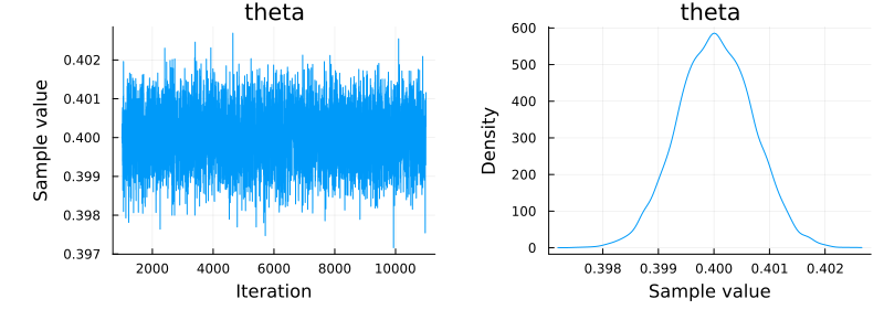
5.6 Recapturing planes
k \sim \text{Hypergeometric}(n, x, t) t \sim \text{Categorical}(\alpha)
x = 10  # number of captures
k = 4  # number of recaptures from n
n = 5  # size of second sample
tmax = 50  # maximum population size

lower = x + (n - k)
upper = tmax

bin_categorial = length(lower:upper)

@model function RecapturingPlanes(k)
    t ~ DiscreteUniform(lower, upper)
    k ~ Hypergeometric(x, t - x , n)
end

iterations=10_000
burnin=1000

recapturing_planes = RecapturingPlanes(k)
chain = sample(recapturing_planes, SMC(), iterations, burnin=burnin)
Sampling: 100%|█████████████████████████████████████████| Time: 0:00:00
Chains MCMC chain (10000×3×1 Array{Float64, 3}):
Log evidence = -2.2807174322546118
Iterations = 1:1:10000
Number of chains = 1
Samples per chain = 10000
Wall duration = 11.31 seconds
Compute duration = 11.31 seconds
parameters = t
internals = lp, weight
Summary Statistics
parameters mean std naive_se mcse ess rhat ⋯
Symbol Float64 Float64 Float64 Float64 Float64 Float64 ⋯
t 17.1500 6.7442 0.0674 0.0860 5737.4943 1.0000 ⋯
1 column omitted
Quantiles
parameters 2.5% 25.0% 50.0% 75.0% 97.5%
Symbol Float64 Float64 Float64 Float64 Float64
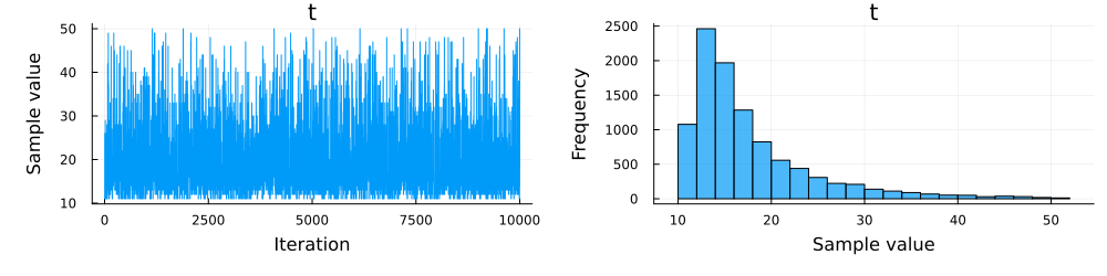
t 11.0000 13.0000 15.0000 19.0000 37.0000